2D Active Fluid

A Two Dimensional Active Fluid Solver

• 

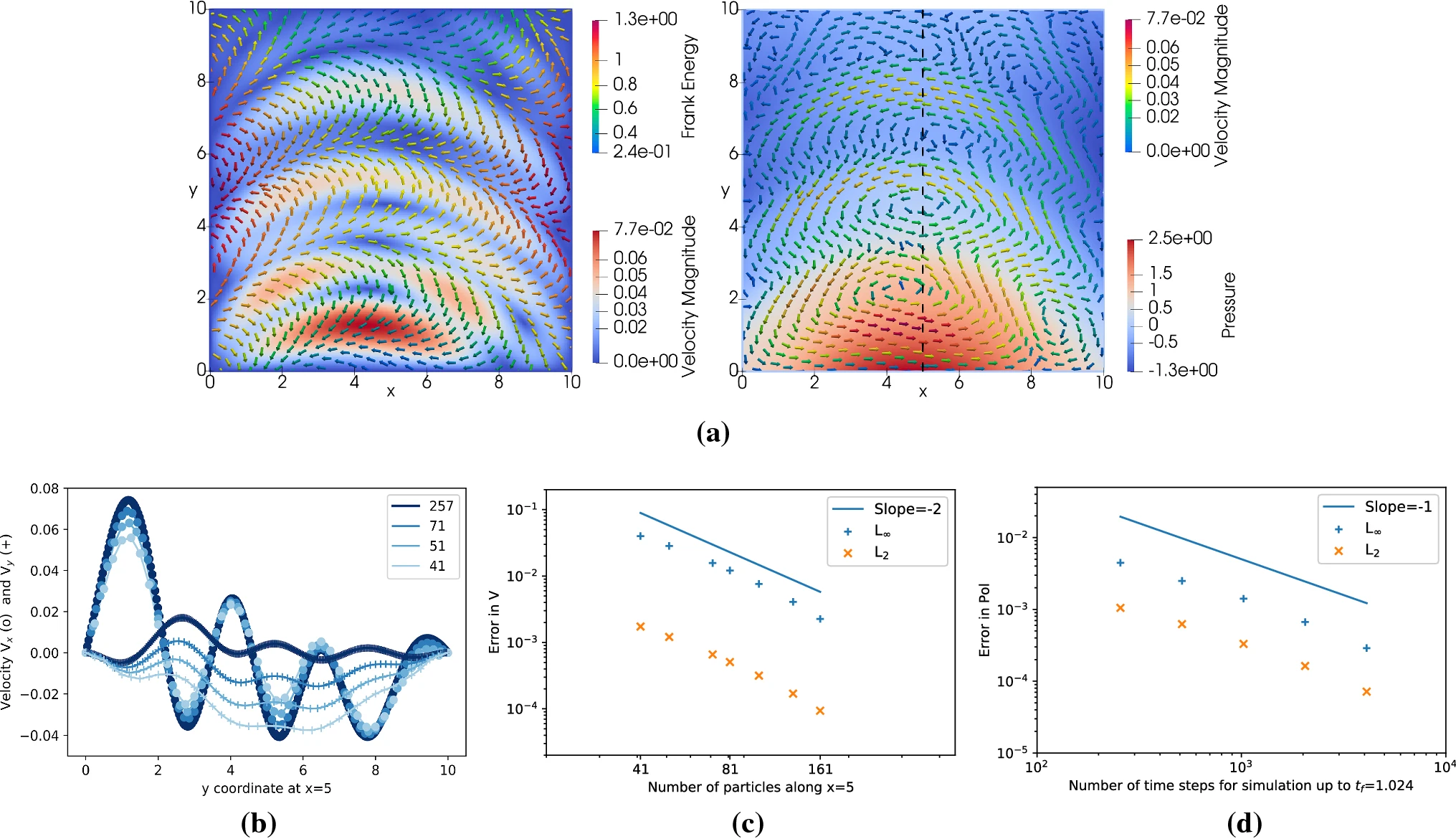
In this example, we perform time integration in a 2d domain of particles of the following Active Fluid partial differential equation:

\[ \frac{\mathrm{D} p_{\alpha}}{\mathrm{D} t}=\frac{h_{\alpha}}{\gamma}-\nu u_{\alpha \beta} p_{\beta}+\lambda\Delta\mu p_\alpha+ \omega_{\alpha \beta} p_{\beta}\\ \partial_{\beta} \sigma_{\alpha \beta}-\partial_{\alpha} \Pi=0 \\ \partial_{\gamma} v_{\gamma}=0\\ 2 \eta u_{\alpha \beta}=\sigma_{\alpha \beta}^{(s)}+\zeta \Delta \mu\left(p_{\alpha} p_{\beta}-\frac{1}{2} p_{\gamma} p_{\gamma} \delta_{\alpha \beta}\right) -\frac{\nu}{2}\left(p_{\alpha} h_{\beta}+p_{\beta} h_{\alpha}-p_{\gamma} h_{\gamma} \delta_{\alpha \beta}\right) \]

It is highly recommended to go through the Odeint Example and the Pressure correction Stokes-Flow example to understand this code.

We employ a Lagrangian frame of reference for polarity time evolution. Hence the PDE is transformed to a system of PDEs:

\[\begin{align} \frac{\partial\vec{X}}{dt}=\vec{V}\\ \frac{\partial p_\alpha}{dt}=\frac{h_{\alpha}}{\gamma}-\nu u_{\alpha \beta} p_{\beta}+\lambda\Delta\mu p_\alpha+ \omega_{\alpha \beta} p_{\beta} \end{align} \]

Where \(\vec{X}\) is the position vector. Hence, we have decoupled the moving of the particles from the evolution of the Polarity. As it can be expensive to recompute derivatives at every stage of a time integrator in a single step, we will integrate the PDEs with seperate techniques (Euler step for moving the particles and solving the force balance for advection).

Output: Time series data of the PDE Solution.

Including the headers

These are the header files that we need to include:

Initialization of the global parameters

We start with

• Initializing certain global parameteres we will use: such as x,y to refer to the dimensions 0 and 1. (Makes it easier to read equations in code)
• Creating empty pointers for coupling openfpm distributed vector with odeint. One for the entire distributed vector and another for the subset or bulk. We seperate bulk and the entire distribution as it makes it easier to impose boundary conditions. (Which will be more apparant in ComputeRHS of the PDE) Note that a subset expression always comes at the left hand side of a computation. (The semantics of the expressions is by denoting what we want to update from regular expressions)

Creating aliases of the types of the datasructures we are going to use in OpenFPM. Property_type as the type of properties we wish to use. dist_vector_type as the 2d openfpm distributed vector type dist_vector_type as the 2d openfpm distributed subset vector type

Creating the RHS Functor

Odeint works with certain specific state_types. We offer certain state types such as 'state_type_2d_ofp' for making openfpm work with odeint.

Now we create the RHS functor. Please refer to ODE_int for more detials. Note that we have templated it with two operator types DXX and DYY as we need to compute Laplacian at each stage. We will pass the DCPSE operators to an instance of this functor.

All RHS computations needs to happen in the operator (). Odeint expects the arguments here to be an input state_type X, an output state_tyoe dxdt and time t. We pass on the openfpm distributed state types as void operator()( const state_type_2d_ofp &X , state_type_2d_ofp &dxdt , const double t ) const

Since we would like to use openfpm here. We cast back the global pointers created before to access the Openfpm distributed vector here. (Note that these pointers needs to initialized in the main(). Further, 'state_type_2d_ofp' is a temporal structure, which means it does not have the ghost. Hence we copy the current state back to the openfpm vector from the openfpm state type X. We do our computations as required. Then we copy back the output into the state_type dxdt)

Creating the Observer Functor

There are multiple ways in which the system can be integrated. For example, and ideally, we could put both the PDEs into the RHS functor (Moving the particles at every stage). This can be expensive. However, Often in numerical simulations, Both the PDEs can be integrated with seperate steppers. To achieve this we will use the observer functor. The observer functor is called before every time step evolution by odeint. Hence we can use it to update the position of the particles, with an euler step. and also update the operators and solve the force balance equations below.

\[ \eta \partial_{x}^{2} v_{\mathrm{x}}+\eta \partial_{y}^{2} v_{\mathrm{x}}-\partial_{x} \Pi+\frac{\nu}{2} \partial_{x}\left[\frac{\gamma \nu u_\mathrm{x x} p_{\mathrm{x}}^{2}\left(p_{\mathrm{x}}^{2}-p_{\mathrm{y}}^{2}\right)}{p_{\mathrm{x}}^{2}+p_{\mathrm{y}}^{2}}\right]+ \frac{\nu}{2} \partial_{x}\left[\frac{2 \gamma \nu u_{\mathrm{xy}} p_{\mathrm{x}} p_{\mathrm{y}}\left(p_{\mathrm{x}}^{2}-p_{\mathrm{y}}^{2}\right)}{p_{\mathrm{x}}^{2}+p_{\mathrm{y}}^{2}}\right] +\frac{\nu}{2} \partial_{x}\left[\frac{\gamma \nu u_{\mathrm{yy}} p_{\mathrm{y}}^{2}\left(p_{\mathrm{x}}^{2}-p_{\mathrm{y}}^{2}\right)}{p_{\mathrm{x}}^{2}+p_{\mathrm{y}}^{2}}\right] + \frac{\nu}{2} \partial_{y}\left[\frac{2 \gamma \nu u_{\mathrm{xx}} p_{\mathrm{x}}^{3} p_{\mathrm{y}}}{p_{\mathrm{x}}^{2}+p_{\mathrm{y}}^{2}}\right]+\frac{\nu}{2} \partial_{y}\left[\frac{4 \gamma \nu u_{\mathrm{xy}} p_{\mathrm{x}}^{2} p_{\mathrm{y}}^{2}}{p_{\mathrm{x}}^{2}+p_{\mathrm{y}}^{2}}\right]+\frac{\nu}{2} \partial_{y}\left[\frac{2 \gamma \nu u_{\mathrm{yy}} p_{\mathrm{x}} p_{\mathrm{y}}^{3}}{p_{\mathrm{x}}^{2}+p_{\mathrm{y}}^{2}}\right] \\ =-\frac{1}{2} \partial_{y}\left(h_{\perp}\right)+\zeta \partial_{x}\left(\Delta \mu p_{\mathrm{x}}^{2}\right)+\zeta \partial_{y}\left(\Delta \mu p_{\mathrm{x}} p_{\mathrm{y}}\right)- \zeta \partial_{x}\left(\Delta \mu \frac{p_{\mathrm{x}}^{2}+p_{\mathrm{y}}^{2}}{2}\right)- \frac{\nu}{2} \partial_{x}\left(-2 h_{\perp} p_{\mathrm{x}} p_{\mathrm{y}}\right) - \quad \frac{\nu}{2} \partial_{y}\left[h_{\perp}\left(p_{\mathrm{x}}^{2}-p_{\mathrm{y}}^{2}\right)\right]-\partial_{x} \sigma_{\mathrm{xx}}^{(\mathrm{e})}-\partial_{y} \sigma_{\mathrm{xy}}^{(\mathrm{e})} + \quad \frac{\nu}{2} \partial_{x}\left[\gamma \lambda \Delta \mu\left(p_{\mathrm{x}}^{2}-p_{\mathrm{y}}^{2}\right)\right]-\frac{\nu}{2} \partial_{y}\left(-2 \gamma \lambda \Delta \mu p_{\mathrm{x}} p_{\mathrm{y}}\right), \\ \eta \partial_{x}^{2} v_{\mathrm{y}}+\eta \partial_{y}^{2} v_{\mathrm{y}}-\partial_{y} \Pi+\frac{\nu}{2} \partial_{y}\left[\frac{-\gamma \nu u_{\mathrm{xx}} p_{\mathrm{x}}^{2}\left(p_{\mathrm{x}}^{2}-p_{\mathrm{y}}^{2}\right)}{p_{\mathrm{x}}^{2}+p_{\mathrm{y}}^{2}}\right] + \frac{\nu}{2} \partial_{y}\left[\frac{-2 \gamma \nu u_{\mathrm{xy}} p_{\mathrm{x}} p_{\mathrm{y}}\left(p_{\mathrm{x}}^{2}-p_{\mathrm{y}}^{2}\right)}{p_{\mathrm{x}}^{2}+p_{\mathrm{y}}^{2}}\right] +\frac{\nu}{2} \partial_{y}\left[\frac{-\gamma \nu u_{\mathrm{yy}} p_{\mathrm{y}}^{2}\left(p_{\mathrm{x}}^{2}-p_{\mathrm{y}}^{2}\right)}{p_{\mathrm{x}}^{2}+p_{\mathrm{y}}^{2}}\right] + \frac{\nu}{2} \partial_{x}\left[\frac{2 \gamma \nu u_{\mathrm{x} x} p_{\mathrm{x}}^{3} p_{\mathrm{y}}}{p_{\mathrm{x}}^{2}+p_{\mathrm{y}}^{2}}\right]+\frac{\nu}{2} \partial_{x}\left[\frac{4 \gamma \nu u_{\mathrm{xx}} p_{\mathrm{x}}^{2} p_{\mathrm{y}}^{2}}{p_{\mathrm{x}}^{2}+p_{\mathrm{y}}^{2}}\right]+\frac{\nu}{2} \partial_{x}\left[\frac{2 \gamma\nu u_{\mathrm{yy}} p_{\mathrm{x}} p_{\mathrm{y}}^{3}}{p_{\mathrm{x}}^{2}+p_{\mathrm{y}}^{2}}\right] \\ =-\frac{1}{2} \partial_{x}\left(-h_{\perp}\right)+\zeta \partial_{y}\left(\Delta \mu p_{\mathrm{y}}^{2}\right)+\zeta \partial_{x}\left(\Delta \mu p_{\mathrm{x}} p_{\mathrm{y}}\right)- \zeta \partial_{y}\left(\Delta \mu \frac{p_{\mathrm{x}}^{2}+p_{\mathrm{y}}^{2}}{2}\right)-\frac{\nu}{2} \partial_{y}\left(2 h_{\perp} p_{\mathrm{x}} p_{\mathrm{y}}\right) - \frac{\nu}{2} \partial_{x}\left[h_{\perp}\left(p_{\mathrm{x}}^{2}-p_{\mathrm{y}}^{2}\right)\right]-\partial_{x} \sigma_{\mathrm{yx}}^{(\mathrm{e})}-\partial_{y} \sigma_{\mathrm{yy}}^{(\mathrm{e})}- \frac{\nu}{2} \partial_{y}\left[\gamma \lambda \Delta \mu\left(p_{\mathrm{x}}^{2}-p_{\mathrm{y}}^{2}\right)\right]-\frac{\nu}{2} \partial_{x}\left(-2 \gamma \lambda \Delta \mu p_{\mathrm{x}} p_{\mathrm{y}}\right). \]

Now we create the Observer functor that will calculate velocity. Note that we have templated it with Differential operators of types DXX and so on. We use them to solve force balance. We further update them after moving the particles.

All Observer computations needs to happen in the operator (). Odeint expects the arguments here to be an input state_type X, and time t. We pass on the openfpm distributed state types as void operator()( const state_type_2d_ofp &X , const double t ) const

Since we would like to use again openfpm here. We cast back the global pointers created before to access the Openfpm distributed vector here. (Note that these pointers needs to initialized in the main(). Further, 'state_type_2d_ofp' is a temporal structure, which means it does not have the ghost. Hence we copy the current state back to the openfpm vector from the openfpm state type X. We do our computations as required. Then we copy back the output into the state_type dxdt.

Initializating OpenFPM

We start with

• Initializing OpenFPM

Creating Particles and assigning subsets

We create a particle distribution we certain rCut for the domain.

Also, we fill the initial Polarity concentration as:

\[ \mathbf{p}(x,y,0)=\left( \begin{matrix} \sin\big(2\pi (\cos\left(\frac{2 x - L_x}{ L_x}\right)-\sin\left(\frac{2 y - L_y}{ L_y}\right) \big)\\[2ex] \cos \big(2\pi (\cos\left(\frac{2 x - L_x}{ L_x}\right)-\sin\left(\frac{2 y - L_y}{ L_y}\right)\big) \end{matrix}\right) \]

Create the subset, differential operators, steppers and Cast Global Pointers

On the particles we just created we need to constructed the subset object based on the numbering. Further, We cast the Global Pointers so that Odeint RHS functor can recognize our openfpm distributed structure.

We create DCPSE based operators and alias the particle properties.

Calling Odeint

We initiliaze the time variable t, step_size dt and final time tf.

We create a vector for storing the intermidiate time steps, as most odeint calls return such an object.

We then Call the Odeint_rk4 method created above to do a rk4 time integration from t0 to tf with arguments as the System, the state_type, current time t and the stepsize dt.

Odeint updates X in place. And automatically advect the particles (an Euler step) and do a map and ghost_get as needed after moving particles by calling the observer.

The observer then updates the subset bulk and the DCPSE operators.

The observer also Solves the Force Balance.

We finally deallocate the DCPSE operators and finalize the library.

Full code