Gray Scott 2D

Solving a gray scott-system

This example show the usage of periodic grid with ghost part given in grid units to solve the following system of equations

\(\frac{\partial u}{\partial t} = D_u \nabla^{2} u - uv^2 + F(1-u)\)

\(\frac{\partial v}{\partial t} = D_v \nabla^{2} v + uv^2 - (F + k)v\)

Constants and functions

First we define convenient constants

constexpr int U = 0;
constexpr int V = 1;

constexpr int x = 0;
constexpr int y = 1;

We also define an init function. This function initialize the species U and V. In the following we are going into the detail of this function

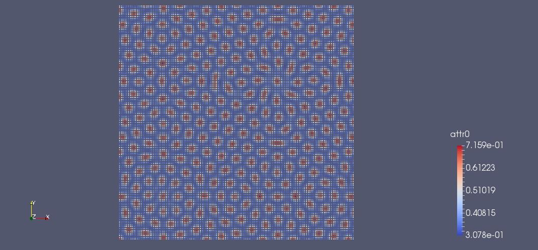
In figure is the final solution of the problem

void init(grid_dist_id<2,double,aggregate<double,double> > & Old, grid_dist_id<2,double,aggregate<double,double> > & New, Box<2,double> & domain)
{

}

Here we initialize for the full domain. U and V itarating across the grid points. For the calculation We are using 2 grids one Old and New. We initialize Old with the initial condition concentration of the species U = 1 over all the domain and concentration of the specie V = 0 over all the domain. While the New grid is initialized to 0

    auto it = Old.getDomainIterator();

    while (it.isNext())
    {
        // Get the local grid key
        auto key = it.get();

        // Old values U and V
        Old.template get<U>(key) = 1.0;
        Old.template get<V>(key) = 0.0;

        // Old values U and V
        New.template get<U>(key) = 0.0;
        New.template get<V>(key) = 0.0;

        ++it;
    }

After we initialized the full grid, we create a perturbation in the domain with different values. We do in the part of space: 1.55 < x < 1.85 and 1.55 < y < 1.85. Or more precisely on the points included in this part of space.

    grid_key_dx<2> start({(long int)std::floor(Old.size(0)*1.55f/domain.getHigh(0)),(long int)std::floor(Old.size(1)*1.55f/domain.getHigh(1))});
    grid_key_dx<2> stop ({(long int)std::ceil (Old.size(0)*1.85f/domain.getHigh(0)),(long int)std::ceil (Old.size(1)*1.85f/domain.getHigh(1))});
    auto it_init = Old.getSubDomainIterator(start,stop);

    while (it_init.isNext())
    {
        auto key = it_init.get();

        Old.template get<U>(key) = 0.5 + (((double)std::rand())/RAND_MAX -0.5)/100.0;
        Old.template get<V>(key) = 0.25 + (((double)std::rand())/RAND_MAX -0.5)/200.0;

        ++it_init;
    }

Initialization

Initialize the library

Create

• A 2D box that define the domain
• an array of 2 unsigned integer that will define the size of the grid on each dimension
• Periodicity of the grid
• A Ghost object that will define the extension of the ghost part for each sub-domain in grid point unit

We also define numerical and physical parameters

• Time stepping for the integration
• Diffusion constant for the species u
• Diffusion constant for the species v
• Number of time-steps
• Physical constant K
• Physical constant F

    openfpm_init(&argc,&argv);

    // domain
    Box<2,double> domain({0.0,0.0},{2.5,2.5});
    
    // grid size
    size_t sz[2] = {128,128};

    // Define periodicity of the grid
    periodicity<2> bc = {PERIODIC,PERIODIC};
    
    // Ghost in grid unit
    Ghost<2,long int> g(1);
    
    // deltaT
    double deltaT = 1;

    // Diffusion constant for specie U
    double du = 2*1e-5;

    // Diffusion constant for specie V
    double dv = 1*1e-5;

    // Number of timesteps
    size_t timeSteps = 15000;

    // K and F (Physical constant in the equation)
    double K = 0.055;
    double F = 0.03;

Here we create 2 distributed grid in 2D Old and New. In particular because we want that the second grid is distributed across processors in the same way we pass the decomposition of the Old grid to the New one in the constructor with Old.getDecomposition(). Doing this, we force the two grid to have the same decomposition.

    grid_dist_id<2, double, aggregate<double,double>> Old(sz,domain,g,bc);

    // New grid with the decomposition of the old grid
    grid_dist_id<2, double, aggregate<double,double>> New(Old.getDecomposition(),sz,g);

    
    // spacing of the grid on x and y
    double spacing[2] = {Old.spacing(0),Old.spacing(1)};

We use the function init to initialize U and V on the grid Old

    init(Old,New,domain);

Time stepping

After initialization, we first synchronize the ghost part of the species U and V for the grid, that we are going to read (Old). In the next we are going to do 15000 time steps using Eulerian integration

Because the update step of the Laplacian operator from \( \frac{\partial u}{\partial t} = \nabla u + ... \) discretized with eulerian time-stepping look like

\( \delta U_{next}(x,y) = \delta t D_u (\frac{U(x+1,y) - 2U(x,y) + U(x-1,y)}{(\delta x)^2} + \frac{U(x,y+1) - 2U(x,y) + U(x,y-1)}{(\delta y)^2}) + ... \)

If \( \delta x = \delta y \) we can simplify with

\( U_{next}(x,y) = \frac{\delta t D_u}{(\delta x)^2} (U(x+1,y) + U(x-1,y) + U(x,y-1) + U(x,y+1) -4U(x,y)) + ... \) (Eq 2)

The specie V follow the same concept while for the \( ... \) it simply expand into

\( - \delta t uv^2 - \delta t F(U - 1.0) \)

and V the same concept

See Also

Ghost

Loop over grid points

Grid coordinates

VTK and visualization

    // sync the ghost
    size_t count = 0;
    Old.template ghost_get<U,V>();

    // because we assume that spacing[x] == spacing[y] we use formula 2
    // and we calculate the prefactor of Eq 2
    double uFactor = deltaT * du/(spacing[x]*spacing[x]);
    double vFactor = deltaT * dv/(spacing[x]*spacing[x]);

    for (size_t i = 0; i < timeSteps; ++i)
    {
        auto it = Old.getDomainIterator();

        while (it.isNext())
        {
            auto key = it.get();

            // update based on Eq 2
            New.get<U>(key) = Old.get<U>(key) + uFactor * (
                                        Old.get<U>(key.move(x,1)) +
                                        Old.get<U>(key.move(x,-1)) +
                                        Old.get<U>(key.move(y,1)) +
                                        Old.get<U>(key.move(y,-1)) +
                                        -4.0*Old.get<U>(key)) +
                                        - deltaT * Old.get<U>(key) * Old.get<V>(key) * Old.get<V>(key) +
                                        - deltaT * F * (Old.get<U>(key) - 1.0);

            // update based on Eq 2
            New.get<V>(key) = Old.get<V>(key) + vFactor * (
                                        Old.get<V>(key.move(x,1)) +
                                        Old.get<V>(key.move(x,-1)) +
                                        Old.get<V>(key.move(y,1)) +
                                        Old.get<V>(key.move(y,-1)) -
                                        4*Old.get<V>(key)) +
                                        deltaT * Old.get<U>(key) * Old.get<V>(key) * Old.get<V>(key) +
                                        - deltaT * (F+K) * Old.get<V>(key);

            // Next point in the grid
            ++it;
        }

        // Here we copy New into the old grid in preparation of the new step
        // It would be better to alternate, but using this we can show the usage
        // of the function copy. To note that copy work only on two grid of the same
        // decomposition. If you want to copy also the decomposition, or force to be
        // exactly the same, use Old = New
        Old.copy(New);

        // After copy we synchronize again the ghost part U and V
        Old.ghost_get<U,V>();

        // Every 100 time step we output the configuration for
        // visualization
        if (i % 100 == 0)
        {
            Old.write_frame("output",count);
            count++;
        }
    }
    

Finalize

Deinitialize the library

    openfpm_finalize();